Introduction to radEmu with TreeSummarizedExperiment
David Clausen, Sarah Teichman and Amy Willis
2026-04-14
Source:vignettes/intro_radEmu_with_tse.Rmd
intro_radEmu_with_tse.RmdFirst, we will install radEmu, if we haven’t
already.
# if (!require("remotes", quietly = TRUE))
#     install.packages("remotes")
#
# remotes::install_github("statdivlab/radEmu")
Next, we can load radEmu as well as the
tidyverse package suite.
Introduction
This vignette provides an introduction to using radEmu
for differential abundance analysis using a
TreeSummarizedExperiment data object. For more in-depth
explanations of how this software works, an example of running
hypothesis tests, and details on this analysis, see the vignette
“intro_radEmu.Rmd”.
In this lab we’ll explore a dataset published by Wirbel et al. (2019). This is a meta-analysis of case-control studies, meaning that Wirbel et al. collected raw sequencing data from studies other researchers conducted and re-analyzed it (in this case, they also collected some new data of their own).
Wirbel et al. published two pieces of data we’ll focus on today:
- metadata giving demographics and other information about participants
- a mOTU (metagenomic OTU) table
In the manuscript, we looked at differential abundance across otherwise similar colorectal cancer and non-cancer control study participants for the 849 mOTUs that Wirbel et al. published. For the purpose of having a streamlined tutorial, we will only look at a subset of those 849 mOTUs in this vignette.
Loading and exploring data
Note that in order to follow along with this tutorial (but not to use
radEmu!) you will need to have
TreeSummarizedExperiment installed. We will check if you
have TreeSummarizedExperiment installed, and if you do not
then you can read the following code but it will not be run.
tse <- requireNamespace("TreeSummarizedExperiment", quietly = TRUE) == TRUE#> [1] "TreeSummarizedExperiment is installed: TRUE"Now that we have loaded the TreeSummarizedExperiment
package, we will create our TreeSummarizedExperiment data
object.
library(TreeSummarizedExperiment)
library(SummarizedExperiment)
library(SingleCellExperiment)
setClassUnion("ExpData", c("matrix", "SummarizedExperiment"))
data(wirbel_sample)
data(wirbel_otu)
data(wirbel_taxonomy)
wirbel_tse <- TreeSummarizedExperiment(assays = list(Count = t(wirbel_otu)),
                                       rowData = wirbel_taxonomy,
                                       colData = wirbel_sample)
wirbel_tse
#> class: TreeSummarizedExperiment
#> dim: 845 566
#> metadata(0):
#> assays(1): Count
#> rownames(845): Streptococcus anginosus [ref_mOTU_v2_0004]
#>   Enterobacteriaceae sp. [ref_mOTU_v2_0036] ... unknown Clostridiales
#>   [meta_mOTU_v2_7795] unknown Clostridiales [meta_mOTU_v2_7800]
#> rowData names(7): domain phylum ... genus species
#> colnames(566): CCIS00146684ST.4.0 CCIS00281083ST.3.0 ... SAMEA3178940
#>   SAMEA3178943
#> colData names(14): Sample_ID External_ID ... BMI_spline.2 Sampling
#> reducedDimNames(0):
#> mainExpName: NULL
#> altExpNames(0):
#> rowLinks: NULL
#> rowTree: NULL
#> colLinks: NULL
#> colTree: NULL
We’ll start by looking at the metadata.
dim(colData(wirbel_tse))
#> [1] 566  14
head(colData(wirbel_tse))
#> DataFrame with 6 rows and 14 columns
#>                             Sample_ID External_ID       Age      Gender
#>                           <character> <character> <integer> <character>
#> CCIS00146684ST.4.0 CCIS00146684ST-4-0      FR-726        72           F
#> CCIS00281083ST.3.0 CCIS00281083ST-3-0      FR-060        53           M
#> CCIS02124300ST.4.0 CCIS02124300ST-4-0      FR-568        35           M
#> CCIS02379307ST.4.0 CCIS02379307ST-4-0      FR-828        67           M
#> CCIS02856720ST.4.0 CCIS02856720ST-4-0      FR-027        74           M
#> CCIS03473770ST.4.0 CCIS03473770ST-4-0      FR-192        29           M
#>                          BMI     Country       Study       Group Library_Size
#>                    <numeric> <character> <character> <character>    <integer>
#> CCIS00146684ST.4.0        25         FRA      FR-CRC         CTR     35443944
#> CCIS00281083ST.3.0        32         FRA      FR-CRC         CTR     19307896
#> CCIS02124300ST.4.0        23         FRA      FR-CRC         CTR     42141246
#> CCIS02379307ST.4.0        28         FRA      FR-CRC         CRC      4829533
#> CCIS02856720ST.4.0        27         FRA      FR-CRC         CTR     34294675
#> CCIS03473770ST.4.0        24         FRA      FR-CRC         CTR     20262319
#>                    Age_spline.1 Age_spline.2 BMI_spline.1 BMI_spline.2
#>                       <numeric>    <numeric>    <numeric>    <numeric>
#> CCIS00146684ST.4.0   -0.1975543     0.738962    1.1898242    -0.560692
#> CCIS00281083ST.3.0   -0.0812613    -0.681853   -1.4067931     2.003914
#> CCIS02124300ST.4.0   -2.1745353    -0.681853    0.4547668    -0.670604
#> CCIS02379307ST.4.0    0.6746432    -0.149048    0.0769882     0.538425
#> CCIS02856720ST.4.0   -0.5464333     1.094166    0.4479336     0.172053
#> CCIS03473770ST.4.0   -2.8722933    -0.681853    0.9526144    -0.670604
#>                       Sampling
#>                    <character>
#> CCIS00146684ST.4.0      BEFORE
#> CCIS00281083ST.3.0      BEFORE
#> CCIS02124300ST.4.0      BEFORE
#> CCIS02379307ST.4.0      BEFORE
#> CCIS02856720ST.4.0      BEFORE
#> CCIS03473770ST.4.0      BEFORE
We can see that this dataset includes observations and variables.
Now let’s look at the mOTU table.
dim(assay(wirbel_tse, "Count"))
#> [1] 845 566
# let's check out a subset
assay(wirbel_tse, "Count")[1:5, 1:3]
#>                                                     CCIS00146684ST.4.0
#> Streptococcus anginosus [ref_mOTU_v2_0004]                           0
#> Enterobacteriaceae sp. [ref_mOTU_v2_0036]                            3
#> Citrobacter sp. [ref_mOTU_v2_0076]                                   0
#> Klebsiella michiganensis/oxytoca [ref_mOTU_v2_0079]                  0
#> Enterococcus faecalis [ref_mOTU_v2_0116]                             0
#>                                                     CCIS00281083ST.3.0
#> Streptococcus anginosus [ref_mOTU_v2_0004]                           0
#> Enterobacteriaceae sp. [ref_mOTU_v2_0036]                            0
#> Citrobacter sp. [ref_mOTU_v2_0076]                                   0
#> Klebsiella michiganensis/oxytoca [ref_mOTU_v2_0079]                  0
#> Enterococcus faecalis [ref_mOTU_v2_0116]                             0
#>                                                     CCIS02124300ST.4.0
#> Streptococcus anginosus [ref_mOTU_v2_0004]                           2
#> Enterobacteriaceae sp. [ref_mOTU_v2_0036]                            5
#> Citrobacter sp. [ref_mOTU_v2_0076]                                   0
#> Klebsiella michiganensis/oxytoca [ref_mOTU_v2_0079]                  0
#> Enterococcus faecalis [ref_mOTU_v2_0116]                             6
We can see that this table has samples (just like the metadata) and mOTUs. Let’s save these mOTU names in a vector.
Finally, we can check out the taxonomy table.
head(rowData(wirbel_tse))
#> DataFrame with 6 rows and 7 columns
#>                                                          domain         phylum
#>                                                     <character>    <character>
#> Streptococcus anginosus [ref_mOTU_v2_0004]             Bacteria      Bacillota
#> Enterobacteriaceae sp. [ref_mOTU_v2_0036]              Bacteria Pseudomonadota
#> Citrobacter sp. [ref_mOTU_v2_0076]                     Bacteria Pseudomonadota
#> Klebsiella michiganensis/oxytoca [ref_mOTU_v2_0079]    Bacteria Pseudomonadota
#> Enterococcus faecalis [ref_mOTU_v2_0116]               Bacteria      Bacillota
#> Lactobacillus salivarius [ref_mOTU_v2_0125]            Bacteria      Bacillota
#>                                                                   class
#>                                                             <character>
#> Streptococcus anginosus [ref_mOTU_v2_0004]                      Bacilli
#> Enterobacteriaceae sp. [ref_mOTU_v2_0036]           Gammaproteobacteria
#> Citrobacter sp. [ref_mOTU_v2_0076]                  Gammaproteobacteria
#> Klebsiella michiganensis/oxytoca [ref_mOTU_v2_0079] Gammaproteobacteria
#> Enterococcus faecalis [ref_mOTU_v2_0116]                        Bacilli
#> Lactobacillus salivarius [ref_mOTU_v2_0125]                     Bacilli
#>                                                                order
#>                                                          <character>
#> Streptococcus anginosus [ref_mOTU_v2_0004]           Lactobacillales
#> Enterobacteriaceae sp. [ref_mOTU_v2_0036]           Enterobacterales
#> Citrobacter sp. [ref_mOTU_v2_0076]                  Enterobacterales
#> Klebsiella michiganensis/oxytoca [ref_mOTU_v2_0079] Enterobacterales
#> Enterococcus faecalis [ref_mOTU_v2_0116]             Lactobacillales
#> Lactobacillus salivarius [ref_mOTU_v2_0125]          Lactobacillales
#>                                                                 family
#>                                                            <character>
#> Streptococcus anginosus [ref_mOTU_v2_0004]            Streptococcaceae
#> Enterobacteriaceae sp. [ref_mOTU_v2_0036]           Enterobacteriaceae
#> Citrobacter sp. [ref_mOTU_v2_0076]                  Enterobacteriaceae
#> Klebsiella michiganensis/oxytoca [ref_mOTU_v2_0079] Enterobacteriaceae
#> Enterococcus faecalis [ref_mOTU_v2_0116]               Enterococcaceae
#> Lactobacillus salivarius [ref_mOTU_v2_0125]           Lactobacillaceae
#>                                                                  genus
#>                                                            <character>
#> Streptococcus anginosus [ref_mOTU_v2_0004]               Streptococcus
#> Enterobacteriaceae sp. [ref_mOTU_v2_0036]           Enterobacteriaceae
#> Citrobacter sp. [ref_mOTU_v2_0076]                         Citrobacter
#> Klebsiella michiganensis/oxytoca [ref_mOTU_v2_0079]         Klebsiella
#> Enterococcus faecalis [ref_mOTU_v2_0116]                  Enterococcus
#> Lactobacillus salivarius [ref_mOTU_v2_0125]              Lactobacillus
#>                                                                    species
#>                                                                <character>
#> Streptococcus anginosus [ref_mOTU_v2_0004]          Streptococcus angino..
#> Enterobacteriaceae sp. [ref_mOTU_v2_0036]           Enterobacteriaceae b..
#> Citrobacter sp. [ref_mOTU_v2_0076]                         Citrobacter sp.
#> Klebsiella michiganensis/oxytoca [ref_mOTU_v2_0079] Klebsiella michigane..
#> Enterococcus faecalis [ref_mOTU_v2_0116]             Enterococcus faecalis
#> Lactobacillus salivarius [ref_mOTU_v2_0125]         Ligilactobacillus sa..
Fitting a model
radEmu is a package that can be used to estimate
fold-differences in the abundance of microbial taxa between levels of a
covariate. In this analysis, the covariate that we are primarily
interested in is whether a sample is from a case of colorectal cancer or
a control. We will make control (“CTR”) the reference category:
While in general we would fit a model to all mOTUs, we are going to subset to some specific genera for the purposes of this tutorial. Let’s look at Eubacterium, Porphyromonas, Faecalibacteria, and Fusobacterium for now.
chosen_genera <- c("Eubacterium", "Faecalibacterium", "Fusobacterium", "Porphyromonas")
genera_rows <- rowData(wirbel_tse)$genus %in% chosen_genera
wirbel_restrict <- wirbel_tse[genera_rows]
Again, while we would generally fit a model using all of our samples, for this tutorial we are only going to consider data from a case-control study from China.
sample_cols <- colData(wirbel_restrict)$Country == "CHI"
wirbel_china <- wirbel_restrict[, sample_cols]
Next, we want to confirm that all samples have at least one non-zero count across the categories we’ve chosen and that all categories have at least one non-zero count across the samples we’ve chosen.
sum(colSums(assay(wirbel_china, "Count")) == 0) # no samples have a count sum of 0
#> [1] 0
sum(rowSums(assay(wirbel_china, "Count")) == 0) # one category has a count sum of 0
#> [1] 1
category_to_rm <- rowSums(assay(wirbel_china, "Count")) == 0
wirbel_china <- wirbel_china[!category_to_rm, ]
sum(rowSums(assay(wirbel_china, "Count")) == 0) # now no categories have a count sum of 0
#> [1] 0
The function that we use to fit our model is called
emuFit. It can accept your data in various forms, and here
we will show how to use it with a TreeSummarizedExperiment
object as input.
ch_fit <- emuFit(formula = ~ Group,
                 Y = wirbel_china,
                 assay_name = "Count",
                 run_score_tests = FALSE)
The way to access estimated coefficients and confidence intervals
from the model is with ch_fit$coef.
Now, we can easily visualize our results using the
plot.emuFit function!
plot(ch_fit)$plots
#> $p1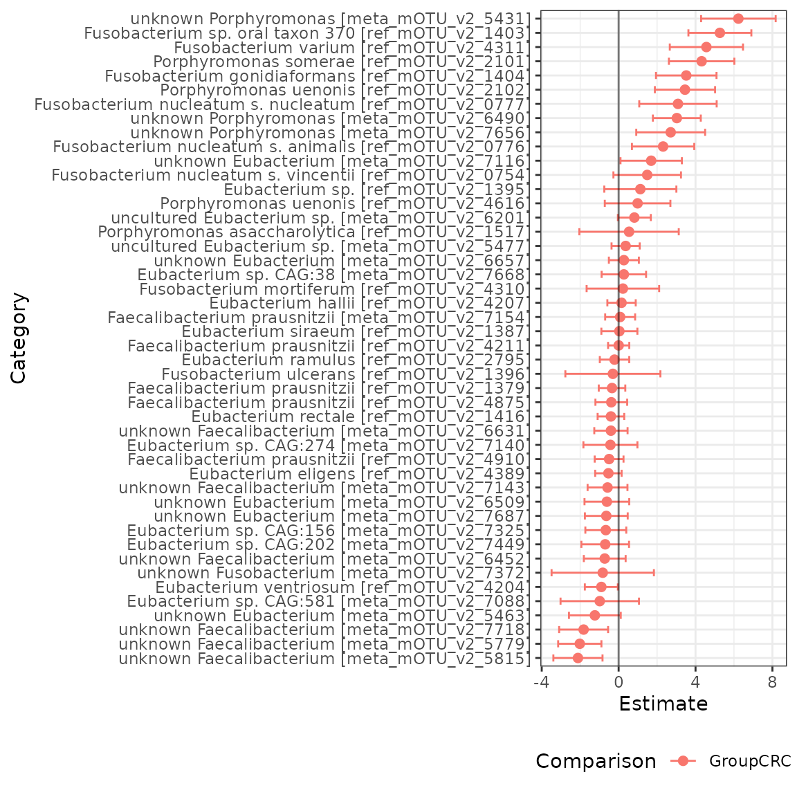
If you’d like to see more explanations of the radEmu
software and additional analyses of this data, check out the vignette
“intro_radEmu.Rmd”.