Comparing detection efficiencies across experiments

Scope and purpose

In this vignette, we will walk through how to use tinyvamp to estimate and compare detection efficiencies across batches or experiments. We will consider the Phase 2 data of Costea et al. (2017), who spiked-in a 10-member synthetic community to 10 samples, which were then sequenced using three shotgun metagenomic sequencing experimental protocols (protocols H, Q and W). Abundances were also measured using flow cytometry.

Specifically, we will demonstrate how to fit the following model: $\begin{align} \text{expected counts for taxon $j$ in sample $i$} = p_{ij} e^{\gamma_i + \beta_{1j} \mathbf{1}_{\{\text{$i$ from sequencing}\}} + \beta_{2j} \mathbf{1}_{\{\text{$i$ from seq. method Q}\}} + \beta_{3j} \mathbf{1}_{\{\text{$i$ from seq. method W}\}} } \end{align}$ where

$p_{i j}$ is the unknown relative abundance of taxon $j$ in sample $i$ . We constrain $\mathbf{p}_i = \mathbf{p}\in \mathbb{S}^{10 - 1}$ for all $i$ , where $\mathbf{p}$ is the composition of the 10-taxa synthetic community spiked into all samples.
$\boldsymbol{\beta}$ reflects differential detection between the four measurement approaches. $\boldsymbol{\beta} \in \mathbb{R}^{3\times10}$ are unknown, with the exception of $\boldsymbol{\beta}_{\cdot 10} = \mathbf{0}_3$ for identifiability. Under this model, $\text{exp}(\beta_{1j})$ , $\text{exp}(\beta_{1j} + \beta_{2j})$ , and $\text{exp}(\beta_{1j} + \beta_{3j})$ give the degree of over- or under-detection of taxon $j$ relative to taxon 10 under protocols H, Q, and W, respectively, using flow cytometry as the reference protocol.

In addition to estimating $\mathbf{p}$ and $\boldsymbol{\beta}$ , we will also test the null hypothesis that detection efficiencies of the three shotgun protocols are the same ( $H_0: \beta_{qj} = 0$ for $q = 2, 3$ and all $j$ ).

Because of its flexibility, fitting a model using tinyvamp involves specifying a lot of parameters. The focus of this vignette will therefore be on how we set up the model to estimate detection efficiencies, rather than why we set up the model in this way. Please see the tinyvamp paper and references therein for those details!

Setup

We will start by loading the relevant packages.

library(tidyverse)
library(tinyvamp)
library(dplyr)
library(ggplot2)
filter <- dplyr::filter

Now let’s load the relevant data and inspect it. This dataset contains the MetaPhlAn2-estimated relative abundances of taxa in 29 samples, formatted in the usual MetaPhlAn2 way (percentages listed at all taxonomic levels):

data("costea2017_metaphlan2_profiles")

Since we are going to compare relative detections of the taxa in the synthetic community that was spiked into all samples, we will start by filtering to only the species in the spiked-in community (10 taxa). To do this, let’s grab the composition data and save the column of species names:

data("costea2017_mock_composition")
mock_taxa <- costea2017_mock_composition$Taxon

Now, we can tidy the MetaPhlAn2 data and pull out the rows for our spike-in species:

costea2017_metaphlan2_profiles_species <- costea2017_metaphlan2_profiles %>% 
  filter(!str_detect(Clade, "t__")) %>% 
  filter(str_detect(Clade, paste(mock_taxa, collapse="|"))) %>% 
  mutate(Clade = str_remove(Clade, ".*s__"))

We can now see our final relative abundance table as follows:

costea2017_metaphlan2_profiles_species
#> # A tibble: 10 × 30
#>    Clade       ERR1971003 ERR1971004 ERR1971005 ERR1971006 ERR1971007 ERR1971008
#>    <chr>            <dbl>      <dbl>      <dbl>      <dbl>      <dbl>      <dbl>
#>  1 Prevotella…    0.837       7.64       6.98      3.14       5.63       0.461  
#>  2 Lactobacil…    0.0944      0.942      0.587     0.655      0.500      0.300  
#>  3 Clostridiu…    0.274       1.47       1.69      0.463      1.81       0.261  
#>  4 Clostridiu…    0.115       0.684      0.441     0.318      0.437      0.117  
#>  5 Blautia_ha…    0.00149     0.0136     0.0117    0.0111     0.00713    0.00315
#>  6 Clostridiu…    0.0325      0.155      0.206     0.0886     0.189      0.0271 
#>  7 Fusobacter…    0.00941     0.0352     0.0822    0.00765    0.0614     0.00724
#>  8 Salmonella…    1.22        6.12       4.20      2.88       3.46       1.77   
#>  9 Yersinia_p…    0.0349      0.266      0.203     0.137      0.141      0.0447 
#> 10 Vibrio_cho…    0.106       0.713      0.452     0.309      0.323      0.0919 
#> # ℹ 23 more variables: ERR1971009 <dbl>, ERR1971010 <dbl>, ERR1971011 <dbl>,
#> #   ERR1971012 <dbl>, ERR1971013 <dbl>, ERR1971014 <dbl>, ERR1971015 <dbl>,
#> #   ERR1971016 <dbl>, ERR1971017 <dbl>, ERR1971018 <dbl>, ERR1971019 <dbl>,
#> #   ERR1971020 <dbl>, ERR1971021 <dbl>, ERR1971022 <dbl>, ERR1971023 <dbl>,
#> #   ERR1971024 <dbl>, ERR1971025 <dbl>, ERR1971026 <dbl>, ERR1971027 <dbl>,
#> #   ERR1971028 <dbl>, ERR1971029 <dbl>, ERR1971030 <dbl>, ERR1971031 <dbl>

Construct observation matrix W

We now need to grab the flow cytometry data and combine it with our sequencing data. Since two observations were taken on all taxa except Vibrio cholerae, let’s start by averaging the flow cytometry measurements, then combining this data with the relative abundance data:

species_by_sample <- costea2017_mock_composition %>% 
  rename(cells_per_ml = 2) %>%
  group_by(Taxon) %>%
  summarize(cells_per_ml = mean(cells_per_ml)) %>%
  inner_join(costea2017_metaphlan2_profiles_species, by = c("Taxon" = "Clade"))

We can then finally arrange our data into the $n \times J$ matrix $\mathbf{W}$ that we will be modeling with tinyvamp:

W <- species_by_sample %>% 
  select(-Taxon) %>% 
  as.matrix %>% 
  t
colnames(W) <- species_by_sample$Taxon

Because it’s a matrix, printing W will display the full observation matrix. Feel free to check it out in an interactive environment!

Specify sample-by-specimen and other design matrices

To fit tinyvamp, we need to specify the detection design matrix $\mathbf{X}$ , which tells the software which samples were sequenced with which protocols. To do that, let’s load the sample data and join it to our abundance data (this makes sure we don’t mix up the order of the rows across datasets):

data("costea2017_sample_data")
protocol_df <- W %>% 
  as_tibble(rownames="Run_accession") %>%
  full_join(costea2017_sample_data) %>% 
  select(Run_accession, Protocol)
#> Joining with `by = join_by(Run_accession)`
protocol_df
#> # A tibble: 30 × 2
#>    Run_accession Protocol
#>    <chr>         <chr>   
#>  1 cells_per_ml  NA      
#>  2 ERR1971003    Q       
#>  3 ERR1971004    Q       
#>  4 ERR1971005    Q       
#>  5 ERR1971006    Q       
#>  6 ERR1971007    Q       
#>  7 ERR1971008    Q       
#>  8 ERR1971009    Q       
#>  9 ERR1971010    Q       
#> 10 ERR1971011    Q       
#> # ℹ 20 more rows

There are lots of different ways we could set up our comparisons between protocols. For example, we could estimate detection efficiencies with respect to the flow cytometry measurements. That is, we could estimate detection effects for protocol H vs flow cytometry; protocol Q vs flow cytometry; protocol W vs flow cytometry (of course, we would get a different estimate of the detection effects for each taxon). That would correspond to this model:

$\begin{align} \text{expected counts for taxon $j$ in sample $i$} = p_{ij} e^{\gamma_i + \beta_{1j} \mathbf{1}_{\{\text{$i$ from seq. method H}\}} + \beta_{2j} \mathbf{1}_{\{\text{$i$ from seq. method Q}\}} + \beta_{3j} \mathbf{1}_{\{\text{$i$ from seq. method W}\}} } \end{align}$

Here’s how we would create that matrix:

X <- protocol_df %>%
  mutate(hh = ifelse(Protocol == "H" & !is.na(Protocol), 1, 0),
         qq = ifelse(Protocol == "Q" & !is.na(Protocol), 1, 0),
         ww = ifelse(Protocol == "W" & !is.na(Protocol), 1, 0)) %>% 
  select(hh, qq, ww) %>%
  as.matrix()   # convert to numeric matrix required by tinyvamp

However, we are interested in assessing the evidence against detection efficiencies being the same between protocols H, Q and W. To make our lives easy for testing this hypothesis later, we’re going to estimate the model slightly differently: we’re going to create a “intercept” variable as well as a protocol Q variable and a protocol W variable. The intercept variable equals 1 for all sequencing protocols, and the Q variable equals 1 for only samples sequenced with the protocol Q and zero for all other samples. You could also think of the intercept as an indicator for “this sample was sequenced”. This is exactly the model we described at the beginning of this vignette:

$\begin{align} \text{expected counts for taxon $j$ in sample $i$} = p_{ij} e^{\gamma_i + \beta_{1j} \mathbf{1}_{\{\text{$i$ from sequencing}\}} + \beta_{2j} \mathbf{1}_{\{\text{$i$ from seq. method Q}\}} + \beta_{3j} \mathbf{1}_{\{\text{$i$ from seq. method W}\}} } \end{align}$

Here’s how we create that matrix:

X <- protocol_df %>%
  mutate(intercept = ifelse(!is.na(Protocol), 1, 0),
         qq = ifelse(Protocol == "Q" & !is.na(Protocol), 1, 0),
         ww = ifelse(Protocol == "W" & !is.na(Protocol), 1, 0)) %>% 
  select(intercept, qq, ww) %>%
  as.matrix

By parameterizing the model this way, we can test whether detection efficiencies being the same between protocols H, Q and W by testing the hypothesis $\beta_{Q\cdot} = \beta_{W\cdot} = \mathbf{0}$ . (This may be clarified below – so if you’re confused, dear reader, read on!)

Since $\mathbf{X}$ and $\boldsymbol{\beta}$ go together in the model, lets also initialize our estimate of $\boldsymbol{\beta}$ , and tell the model what we know about $\boldsymbol{\beta}$ . Let initialize the estimation algorithm at “all taxa have the same detection efficiencies under all protocols”:

J <- ncol(W) ## here, 10
B <- matrix(0, ncol = J, nrow = 3)

(Remember that there are 10 taxa and 3 protocol variables: Intercept, Protocol Q and Protocol W)

What do we know about $\boldsymbol{\beta}$ ? Nothing, right? Well, almost. We always need to choose which taxon we’re comparing our efficiencies against. Let’s choose the last taxon, Yersinia pseudotuberculosis.

B_fixed_indices <- matrix(FALSE, ncol = J, nrow = 3)
B_fixed_indices[, J] <- TRUE

Under this parametrization and constraints, we interpret

$exp\left(\beta_{1j}\right)$ as the degree of multiplicative overdetection of taxon $j$ relative to Yersinia pseudotuberculosis in protocol H compared to flow cytometry
$exp\left(\beta_{2j}\right)$ as the degree of multiplicative overdetection of taxon $j$ relative to Yersinia pseudotuberculosis in protocol Q compared to protocol H
$exp\left(\beta_{3j}\right)$ as the degree of multiplicative overdetection of taxon $j$ relative to Yersinia pseudotuberculosis in protocol W compared to protocol H.

Now let’s move on to set up the sample design matrix, which links samples to specimens. $\mathbf{Z}$ is a $n \times K$ matrix, where $n$ is the number of samples and $K$ is the number of specimens. Here, there is only one specimen – the synthetic community that was spiked-in to every sample. So here’s our $\mathbf{Z}$ :

nn <- nrow(W)
Z <- matrix(1, nrow = nn, ncol = 1)

We now need to initialize our relative abundance matrix $\mathbf{p}$ , a $K \times J$ . Let’s initialize it at the sample relative abundance from the flow cytometry data, and tell the algorithm that we don’t know any of the entries of $\mathbf{p}$ .

P <- matrix(W[1,]/sum(W[1,]), nrow = 1, ncol = J)
P_fixed_indices <- matrix(FALSE, nrow = 1, ncol = J)

Let’s tell tinyvamp that we don’t know the sample intensities $\mathbf{\gamma}$ , and initialize them at the log-total number of reads across all taxa:

gammas <- apply(W,1,function(x) log(sum(x)))
gammas_fixed_indices <- rep(FALSE, length(gammas))

Almost done! We’re not going to try to estimate any contamination in this model – so $\mathbf{\tilde{Z}} = 0$ , $\mathbf{\tilde{X}} = 0$ , $\tilde{\gamma}$ could be anything (we set it to zero), and we tell it “don’t estimate $\mathbf{\tilde{p}}$ ”, like so:

Z_tilde <- matrix(0, nrow= 30, ncol = 1)
Z_tilde_gamma_cols <- 1
gamma_tilde <- matrix(0,ncol = 1, nrow = 1)
gamma_tilde_fixed_indices <- TRUE
P_tilde <- matrix(0,nrow =1, ncol = 10)
P_tilde_fixed_indices <- matrix(TRUE,nrow = 1, ncol = 10)
X_tilde <- matrix(0, ncol = 3, nrow= 1)

Fitting the model

Woohoo! It’s time to fit the model.

full_model <- estimate_parameters(W = W,
                                  X = X,
                                  Z = Z,
                                  Z_tilde = Z_tilde,
                                  Z_tilde_gamma_cols = Z_tilde_gamma_cols,
                                  gammas = gammas,
                                  gammas_fixed_indices = gammas_fixed_indices,
                                  P = P,
                                  P_fixed_indices = P_fixed_indices,
                                  B = B,
                                  B_fixed_indices = B_fixed_indices,
                                  X_tilde = X_tilde,
                                  P_tilde = P_tilde,
                                  P_tilde_fixed_indices = P_tilde_fixed_indices,
                                  gamma_tilde = gamma_tilde,
                                  gamma_tilde_fixed_indices = gamma_tilde_fixed_indices,
                                  alpha_tilde = NULL,
                                  Z_tilde_list = NULL)
full_model$optimization_status
#> [1] "Converged"

Woohoo, done! The model converges quickly (<1 second on my 8 y.o. computer) despite the relatively large number of parameters (67). For this analysis we just use the default optimization settings, but you can play around with them and learn more through ?estimate_parameters

full_model is a list that contains a bunch of information. You can what’s in there with full_model %>% names. Let’s dive right in and check out some of the estimates:

full_model$varying %>% as_tibble
#> # A tibble: 67 × 4
#>     value param     k     j
#>     <dbl> <chr> <dbl> <dbl>
#>  1 0.0343 P         1     1
#>  2 0.106  P         1     2
#>  3 0.0553 P         1     3
#>  4 0.228  P         1     4
#>  5 0.0155 P         1     5
#>  6 0.168  P         1     6
#>  7 0.0688 P         1     7
#>  8 0.147  P         1     8
#>  9 0.0773 P         1     9
#> 10 0.0992 P         1    10
#> # ℹ 57 more rows

Let’s visually compare the sequencing protocols with respect to flow cytometry. We have to be a bit careful here to think about our parametrization: remember that $\text{exp}(\beta_{1j})$ , $\text{exp}(\beta_{1j} + \beta_{2j})$ , and $\text{exp}(\beta_{1j} + \beta_{3j})$ give the degree of over- or under-detection of taxon $j$ relative to taxon 10 under protocols H, Q, and W, respectively, using flow cytometry as the reference protocol. That is, to compare to flow cytometry, we want to look at $\beta_{1j} + \beta_{2j}$ , not just $\beta_{2j}$ . Let’s set that up:

the_settings <- X %>% as_tibble %>% dplyr::distinct()
fitted_detectabilities <- (X %*% full_model$B) %>% as_tibble %>% dplyr::distinct()
#> Warning: The `x` argument of `as_tibble.matrix()` must have unique column names if
#> `.name_repair` is omitted as of tibble 2.0.0.
#> ℹ Using compatibility `.name_repair`.
#> This warning is displayed once per session.
#> Call `lifecycle::last_lifecycle_warnings()` to see where this warning was
#> generated.
colnames(fitted_detectabilities) <- colnames(W)
the_betahats <- the_settings %>% 
  mutate("setting" = ifelse(intercept == 0, "Flow cytometry",
                            ifelse(qq == 0 & ww == 0, "H relative to FC",
                                   ifelse(qq == 1 & ww == 0, "Q relative to FC",
                                          "W relative to FC"))), .before = 1) %>% 
  bind_cols(fitted_detectabilities) %>% 
  select(-intercept, -qq, -ww) %>% 
  pivot_longer(-setting)
the_betahats
#> # A tibble: 40 × 3
#>    setting        name                        value
#>    <chr>          <chr>                       <dbl>
#>  1 Flow cytometry Blautia_hansenii                0
#>  2 Flow cytometry Clostridium_difficile           0
#>  3 Flow cytometry Clostridium_perfringens         0
#>  4 Flow cytometry Clostridium_saccharolyticum     0
#>  5 Flow cytometry Fusobacterium_nucleatum         0
#>  6 Flow cytometry Lactobacillus_plantarum         0
#>  7 Flow cytometry Prevotella_melaninogenica       0
#>  8 Flow cytometry Salmonella_enterica             0
#>  9 Flow cytometry Vibrio_cholerae                 0
#> 10 Flow cytometry Yersinia_pseudotuberculosis     0
#> # ℹ 30 more rows
the_betahats %>% 
  ggplot(aes(x = name, y = value, color = setting)) +
  geom_point() +
  labs(
    y = "Estimated log-detection efficiency\n(relative to Y. pseudotuberculosis)",
    x = "",
  ) + 
  theme_bw() + 
  theme(axis.text.x = element_text(angle = 45, vjust = 1, hjust=1))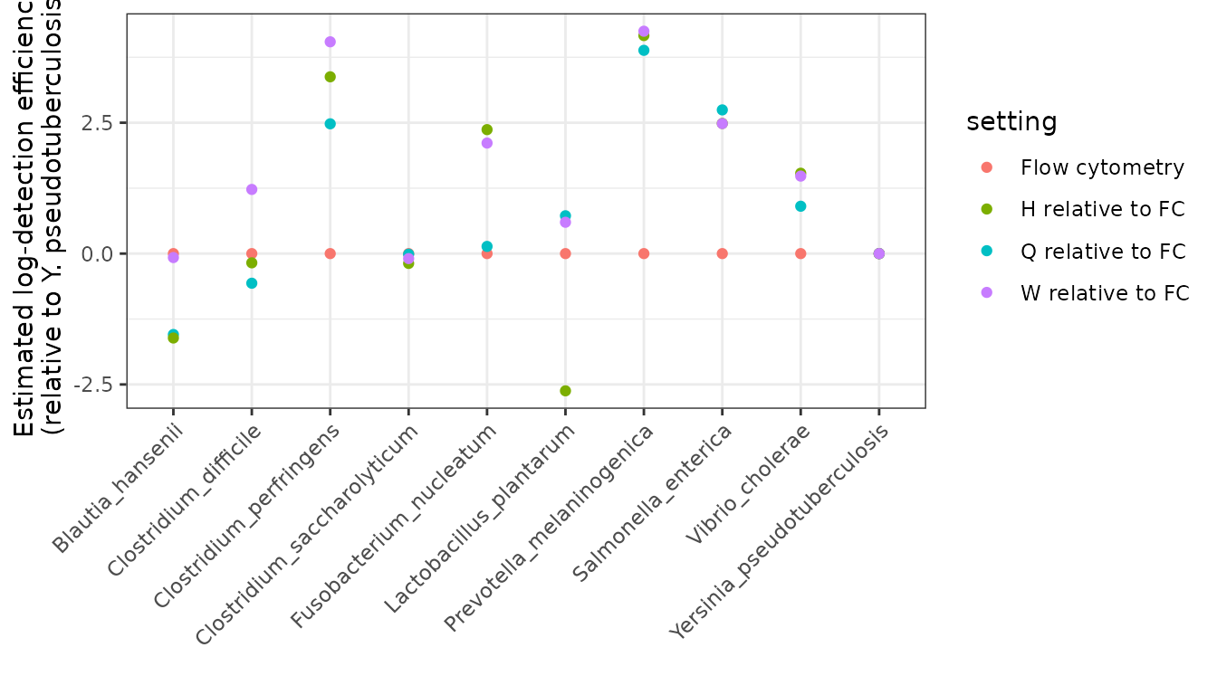

Testing the hypothesis of equal detectability

Testing whether detection efficiencies are identical across protocols H, Q, and W corresponds to the hypothesis $\beta_{Q,j} = \beta_{W,j} = 0$ for all $j = 1, \ldots, J-1$ . In other words, protocols Q and W don’t differ from protocol H in their detectabilities, where the detectabilities are relative to flow cytometry.

To test this hypothesis, we need to tell tinyvamp what the null hypothesis is. We do this as follows:

### Create null model specification for test
null_param <- full_model
### set second and third rows of B equal to zero
null_param$B[2:3,] <- 0
null_param$B_fixed_indices[2:3,] <- TRUE

We then refit the model under the null to obtain the sampling distribution of the test statistics under the null, and compare the observed test statistics to this null distribution. The wall time of this step is proportional to n_boot, but can be parallelized across your computer’s cores using the package parallel. Using only one core, 10 bootstrap iterations took less than 35 seconds on my 1.4 GHz Dual-Core Intel Core i7 from 2017. So, on a more modern machine using parallelization, even 100 iterations should take even less than a minute. Take this minute to stretch your neck and hands, or look at a photo of your favourite cat.

bootstrap_test <-  
  bootstrap_lrt(W = W,
                fitted_model= full_model,
                null_param = null_param,
                n_boot = 500, # do 1000 for a paper, 100 for a first look
                ncores = 5,
                parallelize = TRUE)

You can obtain the p-value for this test via bootstrap_test$boot_pval. Here, it’s definitely rejected – not one bootstrapped test statistic under the null came close to our observed test statistic.

Ok! That’s it for estimation and testing of detectabilities. Let us know your questions, and thanks for using tinyvamp!

References

Costea, P., Zeller, G., Sunagawa, S. et al. Towards standards for human fecal sample processing in metagenomic studies. Nat Biotechnol 35, 1069–1076 (2017). https://doi.org/10.1038/nbt.3960.
Clausen, D.S. and Willis, A.D. Modeling complex measurement error in microbiome experiments. arxiv 2204.12733. https://arxiv.org/abs/2204.12733.

Comparing detection efficiencies across experiments

Amy D Willis and David S Clausen

Scope and purpose